Supervised Learning in R: How to fit a line?

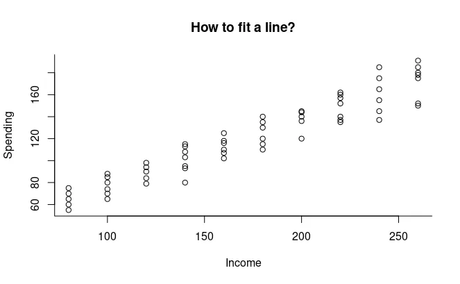
Fitting a line means that the data points are best related to a line. One way to do this is to choose a slope and y-intercept value that defines the line. This slope and y-intercept value will represent the line that is closest to the data points. I believe the power of examples and illustrations. Thus, let's say we have data on the monthly spending(Y) and monthly income(X) of 60 families. These families want to know how much they will spend next month.

X <- c(rep(80,5),rep(100,6),rep(120,5),rep(140,7),        rep(160,6),rep(180,6),rep(200,5),rep(220,7),rep(240,6),rep(260,7)) Y <- c(55,60,65,70,75,65,70,74,80,85,88,79,84,90,94,98,80,93,95,103,108,113,115,        102,107,110,116,118,125,110,115,120,130,135,140,120,136,140,144,145,135,137,        140,152,157,160,162,137,145,155,165,175,185,150,152,175,178,180,185,191)

The first step will be to plot our data points on a graph. We will have income on the X-axis and spending on the Y-axis.

plot(x, y, main="How to fit a line?", xlab="Income", ylab="Spending", bty = "l")

Next, we need to choose the best line. We can try several different lines, but the one that gives the best fit will be the one that is closest to the data points.

To select the best line, we need to determine a slope (m) and y-intercept (b) value. To determine these values, we can use the least squares method. This method calculates the distance of each data point from the line and selects the line that minimizes the sum of the squares of these distances.

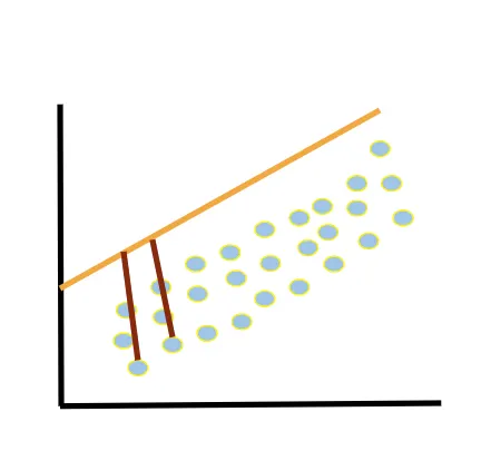
Lets assume that we fit a line like the following:

If you examine the orange line, you will notice that the distance between the orange line and the data points is large.

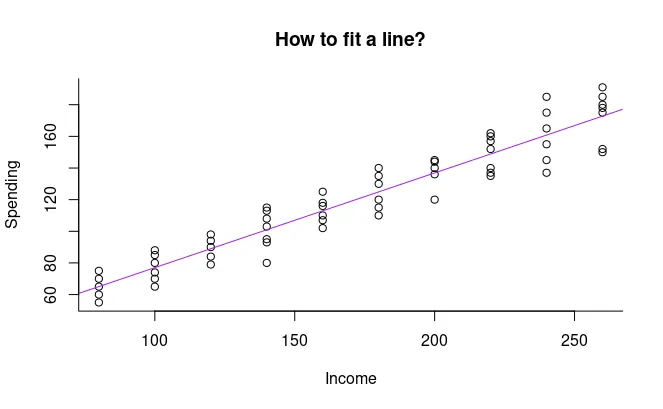
What if we draw a line like the one below?

As you can see, the distance between the pink line and the data points is less. This is how the ordinary least squares method works. The line is drawn with the minimum distance between the data points.

Finally, we can draw the line using the slope and y-intercept values we found. This line will best represent our data. Now, let's do the mathematical calculations behind these illustrations using R.

As I mentioned earlier, the least squares method is used to calculate the best line that can be drawn. For this, a matrix representation of the data points is required.

X <- cbind(rep(1, length(X)), X) Y <- matrix(Y, ncol = 1)

First, the vectors containing the data points are transformed into matrices X and Y. The X matrix is created by adding a column vector next to each value in the x vector. This means that the first column all has the value 1 and the second column has the values in the x vector. The y matrix is a column matrix of the y vector.

Next, the transpose of matrix X is taken. This replaces the columns of the matrix with rows, resulting in a 2x60 matrix. This matrix can be used to access each row of matrix X individually.

XT <- t(X) YT <- t(Y)

The product of matrices is obtained by multiplying the transpose of matrix X by matrix X. This yields a 2x1 matrix and contains the coefficients in the line fit.

XTX <- XT %*% X XTY <- XT %*% Y

In the last step, we calculate the coefficients of the line using the least squares method. The matrix XTX is the sum of squares of our independent variable (x) and the matrix XTY represents the sum of the cross product between our dependent variable (y) and our independent variable. We calculate the coefficients by taking the inverse of the product of these matrices. B[1] represents the y-intercept value and B[2] the slope.

B <- solve(XTX, XTY)

Finally, we can plot the best line.

plot(X[,2], Y, main="How to fit a line?", xlab="Income", ylab="Spending", bty = "l") abline(B, col="purple")

Fitting a line in R

In R, it is not always that hard to draw a line. It can easily be done with lm function.

X <- c(rep(80,5),rep(100,6),rep(120,5),rep(140,7),        rep(160,6),rep(180,6),rep(200,5),rep(220,7),rep(240,6),rep(260,7)) Y <- c(55,60,65,70,75,65,70,74,80,85,88,79,84,90,94,98,80,93,95,103,108,113,115,        102,107,110,116,118,125,110,115,120,130,135,140,120,136,140,144,145,135,137,        140,152,157,160,162,137,145,155,165,175,185,150,152,175,178,180,185,191)  fit <- lm(Y ~ X)

Now, lets draw the line:

plot(X, Y, main="How to fit a line?", xlab="Income", ylab="Spending", bty = "l") abline(fit, col="purple")

This was the first post in a series called Supervised Learning in R. Hope to see you in the next posts,

Just like always:

"In case I don't see ya, good afternoon, good evening, and good night!"