Unsupervised Learning in R: Density Based Clustering
In the previous posts of this series, I covered methods to determine the optimal number of clusters, how k-means , k-medoids, and hierarchical clustering algorithms work in detail. In this fifth post of the Unsupervised Learning in R series, I will try to explain Density Based Clustering algorithm. First, I will explain what Density Based Clustering is, then I will explain how it works step by step, and then I will explain how to implement it using the R program language.
What Density Based Clustering is?
Density-based clustering is a type of clustering algorithm that groups together data points that are closely packed together, while separating those that are more sparsely distributed. The main idea behind density-based clustering is to identify regions in the feature space where the data points are dense, and then to extract clusters based on these regions. [1]
One commonly used density-based clustering algorithm is DBSCAN (Density-Based Spatial Clustering of Applications with Noise). DBSCAN groups together data points that are close to each other based on a distance measure and a density threshold. It defines clusters as dense regions of points that are separated from other dense regions by regions of lower point density. [2]
In density-based clustering, the number of clusters does not need to be predetermined, but the values of MinPts and eps do. Thus, it is important to know what these two parameter means.
The eps parameter defines the radius of the neighbors around a point x. This is called the epsilon neighborhood of x.
The MinPts parameter is the minimum number of neighbors within the “eps” radius. KNN distplot can be used to determine these values.
In the DBSCAN (Density-Based Spatial Clustering of Applications with Noise) algorithm, there are three types of points: core points, border points, and noise points.
-
A core point is a point that has at least MinPts within its epsilon neighborhood. In other words, a core point has enough nearby neighbors to be considered as part of a cluster.
-
A border point is a point that is not a core point, but it is within the epsilon neighborhood of a core point. Border points can be considered as part of a cluster, but they are not as strongly connected to the cluster as core points.
-
A noise point is a point that does not have any core points within its epsilon neighborhood. Noise points are often considered outliers and are not part of any cluster.
Step by Step
Here are the steps involved in the DBSCAN algorithm:
-
The first step is to define epsilon.
-
Identify MinPts.
-
Identify border points: A border point is a point that has fewer than MinPts within its epsilon neighborhood, but is reachable from a core point. These points are often considered part of a cluster but can also be considered noise.
-
Starting with a core point, the algorithm finds all the points within its epsilon neighborhood and assigns them to the same cluster. It then repeats this process for each core point and continues to add points to the same cluster as long as they are within epsilon distance of another point in the cluster.
-
Output clusters: The algorithm outputs the clusters that have been identified.
The following gif is beneficial to understand how DBSCAN works:
https://cdn-images-1.medium.com/max/800/1*GxaDEsIpj-xbElZVPZH0Hg.gif
Just like other clustering algorithms, the DBSCAN algorithm has some advantages and disadvantages. Some of these advantages can be listed as follows:
-
Density-based clustering algorithms can handle noisy data since they can identify noise points as outliers that do not belong to any cluster.
-
Unlike some other clustering algorithms, density-based clustering can identify clusters of different shapes and sizes, including irregularly shaped clusters.
-
Density-based clustering algorithms can automatically determine the number of clusters present in the data, rather than relying on the user to specify the number of clusters.
-
Density-based clustering can be very efficient for large datasets. However, this has an important issue that will be mentioned in the disadvantages.
Some of the disadvantages can be listed as follows:
-
Density-based clustering algorithms have some parameters that need to be set manually, such as epsilon and MinPts, and the choice of these parameters can have a significant impact on the clustering results.
-
Density-based clustering algorithms struggle to handle clusters that have varying densities. If the density of a cluster changes significantly within the cluster or between clusters, it can be difficult for the algorithm to identify the clusters accurately.
-
Density-based clustering algorithms typically require more memory than some other clustering algorithms, especially when dealing with high-dimensional datasets.
-
Density-based clustering algorithms can be less effective on datasets with high dimensionality or large numbers of features, as they suffer from the “curse of dimensionality” which can make it difficult to identify meaningful clusters.
Overall, density-based clustering algorithms can be very effective for many clustering tasks, especially when the data has varying densities and shapes. However, it is important to carefully tune the parameters and consider the limitations of the algorithm when applying it to a particular dataset.
Density Based Clustering in R
Just like other clustering algorithms, DBSCAN can be done quite simply through R. There must be other packages, but I will share with you the dbscan function in the fpc package. I will again use the same dataset, Breast Cancer Wisconsin from the UCI Machine Learning Repository in the analysis.
As I said before, in density-based clustering, the number of clusters does not need to be predetermined, but the values of MinPts and eps do. This is why, as a first step we will draw a kNN distplot to decide these parameters.
kNNdistplot(pcadata, k = 10)
abline(h = 1, lty = 2)
abline(h = 0.6, lty = 2)
In the code, k stands for MinPts. After several trials, 10 was decided upon. When analyzing the kNNdisplot, just like the Elbow Method, the point where the line makes an “elbow” should be determined. This point should be chosen as the eps value. After various trials, the most appropriate value was decided to be 0.6.
In the analysis with minPts 10, eps 1, the number of clusters was found to be one. Since one cluster means no cluster, it was decided not to include it in the post.
The analysis with MinPts 10, eps 0.8 gave the same result as the analysis with eps 1, so it was decided not to include it in the post.
In the analysis with minPts 5, eps 0.6, the number of clusters was two. While there were 513 observations in the first cluster, the number of observations in the second cluster was 7 and the variance differences caused by this imbalance caused suspicion. For this reason, it was not included in the post.
Having decided on the epsilon and Minpts values, we can now apply DBSCAN with these parameters.
db <- fpc::dbscan(df, eps = 0.6, MinPts = 10)
print(db)
dbscan Pts=569 MinPts=10 eps=0.6 0 1 2 border 96 58 27 seed 0 49 339 total 96 107 366
If we analyse the output, we can make the following comments:
-
Density-based clustering divided the dataset into two clusters.
-
The output shows a total of 96 noise values which cannot be assigned to any cluster.
-
There are 58 border points in the first cluster and 27 in the second cluster.
-
There are 49 seed points in the first cluster and 339 seed points in the second cluster.
Just as we did in the previous clustering algorithms, we can also visualize cluster graph with fviz_cluster function in the factoextra package:
fviz_cluster(db, data = df, stand = FALSE, ellipse = FALSE, show.clust.cent = FALSE, geom = "point",palette = "jco", ggtheme = theme_classic())
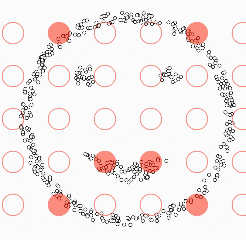
When the plot is examined, it can be seen that the observation difference between the clusters is small. The excess of noise values(black points) is also noteworthy.
That was the end of this post. Just like always:
“In case I don’t see ya, good afternoon, good evening, and good night!”
References
[1] Kriegel, H. P., Kröger, P., Sander, J., & Zimek, A. (2011). Density‐based clustering. Wiley interdisciplinary reviews: data mining and knowledge discovery, 1(3), 231–240.
[2] Bäcklund, H., Hedblom, A., & Neijman, N. (2011). A density-based spatial clustering of application with noise. Data Mining TNM033, 33, 11–30.