In the previous posts of this series, I covered methods to determine the optimal number of clusters, how k-means and k-medoids clustering algorithms work in detail. In this post, I will try to explain Hierarchical Clustering algorithm. First, I will explain what Hierarchical Clustering is, then I will explain how it works step by step, and then I will explain how to implement it using the R program language.
What Hierarchical Clustering is?
Hierarchical Clustering is a method of clustering in which the objects are organized into a tree-like structure called a dendrogram. The main idea behind hierarchical clustering is to start with each object as a separate cluster and then combine them into larger clusters iteratively based on their similarity. There are two main types of hierarchical clustering: Agglomerative and Divisive. [1], [2], [3]
Step by Step — Agglomerative Hierarchical Clustering
-
Start with each object as a separate cluster
-
Find the two most similar clusters and combine them into a new cluster
-
Repeat step 2 until all objects are in the same cluster
Step by Step — Divisive Hierarchical Clustering
-
Start with all objects in the same cluster
-
Divide the largest cluster into two smaller clusters based on their similarity
-
Repeat step 2 until each object forms its own cluster
In hierarchical clustering, there are several linkage methods that can be used to determine the distance between clusters. These linkage methods include:
-
Single linkage: Also known as the nearest-neighbor method, this method calculates the distance between the closest points of the two clusters being merged. [4]
-
Complete linkage: Also known as the farthest-neighbor method, this method calculates the distance between the furthest points of the two clusters being merged.[5]
-
Average linkage: This method calculates the average distance between all pairs of points in the two clusters being merged. [6]
-
Ward’s Minimum Variance linkage: This method minimizes the variance of the distances between points within the same cluster. It merges the clusters that result in the smallest increase in the total sum of squared distances within each cluster.[7]
The choice of linkage method can have a significant impact on the resulting clusters, as each method has its own strengths and weaknesses. Therefore, it is important to carefully consider which linkage method is most appropriate for the data and the specific problem being addressed. In this post, I will focus on two metrics which are Ward’s Minimum Variance Method and Average linkage method.
Ward’s Minimum Variance Method
Ward linkage is a hierarchical clustering method that aims to minimize the variance of the distances between points within the same cluster. It merges the clusters that result in the smallest increase in the total sum of squared distances within each cluster.
To understand how Ward linkage works, let’s assume we have n data points and we start with each point in its own cluster. At each step, we merge the two clusters that result in the smallest increase in the total sum of squared distances within each cluster.
To measure the increase in the total sum of squared distances within each cluster, we use the following formula:

The first step in Ward linkage is to calculate the centroids of each individual point, since each point starts as its own cluster. Then, we calculate the pairwise distances between each centroid. Next, we merge the two clusters with the smallest value of the total sum of squared, and calculate the new centroid of the merged cluster. We repeat this process until all the points are in a single cluster.
As I said in the previous post, there are lots of distance metrics that are used in clustering analysis. In the case of Hierarchical Clustering, there is a way to decide distance metric which is called cophenetic distance.
Cophenetic Distance
The cophenetic distance is a measure used in hierarchical clustering to evaluate the similarity between two observations in the dendrogram produced by the clustering algorithm. It is defined as the distance between two observations in the original data space at the level in the dendrogram where they first merge into the same cluster[8].
The cophenetic distance is calculated as follows:
-
Perform hierarchical clustering on the data to produce a dendrogram
-
For each pair of observations, find the level in the dendrogram where they first merge into the same cluster.
-
Compute the distance between the two observations in the original data space. Repeat steps 2 and 3 for all pairs of observations.
The cophenetic distance is used to evaluate the quality of the clustering solution by comparing it to the original data space. A high correlation between the cophenetic distance and the original distance between observations in the data space indicates that the clustering solution is preserving the structure of the data well.
Cophenetic Distance in R
There are many packages and functions available to implement the k-means algorithm in R. In this article, I will show you the cophenetic function in thestatspackage. I will again use the same dataset, Breast Cancer Wisconsin from the UCI Machine Learning Repository in the analysis.
At first, we need to calculate Euclidean and Manhattan distances between observations:
dist_euc <- dist(pcadf, method="euclidean") # data, distance metric
dist_man <- dist(pcadf, method="manhattan") # data, distance metric
Secondly, we need to hierarchically cluster dataset with both distance metric.
hc_e <- hclust(d=dist_euc, method="ward.D2")
hc_m <- hclust(d=dist_man, method="ward.D2")
Lastly, we need to calculate cophenetic distance for both of the clusterings, and check the correlation coefficient between distance metric and cophenetic distance.
# for euclidean distance
coph_e <- cophenetic(hc_e)
cor(dist_euc,coph_e)

# for manhattan distance
coph_m <- cophenetic(hc_m)
cor(dist_man,coph_m)
> cor(dist_euc,coph_e)
[1] 0.6711685

> cor(dist_man,coph_m)
[1] 0.6018289
In general, a higher cophenetic correlation coefficient indicates that the dendrogram is a more accurate representation of the pairwise distances between the original data points. The cophenetic correlation coefficient can range between 0 and 1, with a value of 1 indicating a perfect fit between the dendrogram and the pairwise distances.
In this case it can be said that when the correlation between Cophenetic and distance matrix is examined, it is observed that hierarchical clustering with Euclidean distance gives better results. That’s why I will continue the analysis with Euclidean distance metric.
Ward’s Minimum Variance Method in R
Hierarchical clustering can be represented by a dendrogram, which is a tree-like structure that shows the hierarchy of clusters and the relations between them. The dendrogram can be cut at a certain height to obtain a flat clustering solution with a specific number of clusters. To determine the number of clusters, as we did in the k-means and k-medoids, we can use methods to determine the optimal number of clusters.
Since I covered methods to determine the optimal number of clusters in the first post of this series, I will not show you the codes in this post. However, I can state that all of the methods suggested 2 as the optimal number of cluster.
As I mentioned, another way for hierarchical clustering is to check the dendogram to decide where to cut it in order to decide the optimal number of cluster. However, I, personally, find this method “open-ended” which I do not think it to be a case for the optimal number of cluster. Nevertheless, I will share codes and dendogram with you.
You can use fviz_dend function in the factoextra package to visualise dendogram of a hierarchical clustering with the object you created from hierarchical clustering with the function hclust from stats package.
hc_e <- hclust(d=dist_euc, method="ward.D2")
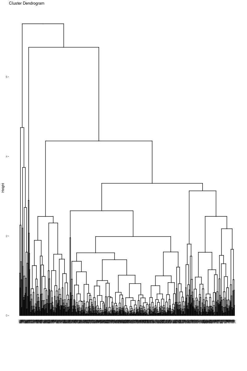
fviz_dend(hc_e,cex=.5)

According to the dendogram, it can be said that the best height value to cut the dendogram is 35–40. This also refers to 2 clusters. Lets hierarchically cluster the data set with 2 clusters. I will use cutree function from the stats package to do that.
grupward2 <- cutree(hc_e, k = 2)
table(grupward2) # gives observation number in each cluster
grupward2 # gives cluster assignments for each observation
grupward2
  1   2
180 389
> grupward2
  [1] 1 1 1 1 1 1 1 1 1 1 2 2 1 2 1 1 2 1 1 2 2 2 1 1 1 1 1 1 1 1 1 1 1 1 1 1 2
 [38] 2 2 2 2 1 1 1 2 1 2 1 2 2 2 2 2 1 2 2 1 1 2 2 2 2 1 2 1 1 2 2 1 2 1 2 1 2
 [75] 2 2 1 1 1 2 2 1 1 1 2 1 2 1 2 1 2 2 2 2 1 1 2 2 2 2 2 2 2 2 2 1 2 2 1 2 2
[112] 2 1 2 2 2 2 1 1 2 2 1 1 2 2 2 2 2 1 1 2 2 2 2 1 2 2 2 1 2 2 2 2 2 2 2 1 2
[149] 2 2 2 2 1 2 2 2 1 2 2 2 2 1 1 2 1 2 2 2 1 2 2 2 1 2 2 2 2 1 2 2 1 1 2 2 2
[186] 2 2 2 2 2 1 2 2 1 1 2 1 2 1 2 2 2 1 1 2 2 2 2 1 2 1 2 1 1 2 1 2 2 1 1 2 2
[223] 2 2 2 2 2 2 2 1 1 2 2 1 2 2 1 1 2 1 2 2 2 2 1 2 2 2 2 2 1 2 1 1 1 2 1 1 1
[260] 1 1 2 1 2 1 1 2 2 2 2 2 2 1 2 2 2 2 2 2 2 1 2 1 1 2 2 2 2 2 2 2 2 2 2 2 2
[297] 2 2 2 2 1 2 1 2 2 2 2 2 2 2 2 2 2 2 2 2 2 1 1 2 2 1 2 1 2 2 2 2 1 1 2 2 2
[334] 2 2 1 2 1 2 1 2 2 2 1 2 2 2 2 2 2 2 1 1 2 2 2 1 2 2 2 2 2 2 2 2 1 1 2 1 1
[371] 1 2 1 1 2 2 1 2 2 1 2 2 2 2 2 2 2 2 2 1 2 2 1 1 2 2 2 2 2 2 1 2 2 2 2 2 2
[408] 2 1 2 2 2 2 2 2 2 2 1 2 2 2 1 2 2 2 2 2 2 2 2 1 2 1 1 2 2 2 2 2 2 2 2 2 2
[445] 1 2 1 2 2 1 2 1 2 2 2 2 2 2 2 2 1 1 2 2 2 2 2 2 1 1 2 2 2 2 2 2 2 2 2 1 2
[482] 2 2 2 2 1 2 1 2 2 2 2 1 2 2 2 2 2 1 1 2 1 2 1 1 1 2 2 2 1 2 2 1 2 2 2 1 1
[519] 1 2 2 1 2 2 2 2 2 2 1 2 2 2 2 1 2 1 2 1 2 2 2 2 2 2 2 2 2 2 2 2 2 2 2 2 2
[556] 2 2 2 2 2 2 2 1 1 1 1 2 1 2
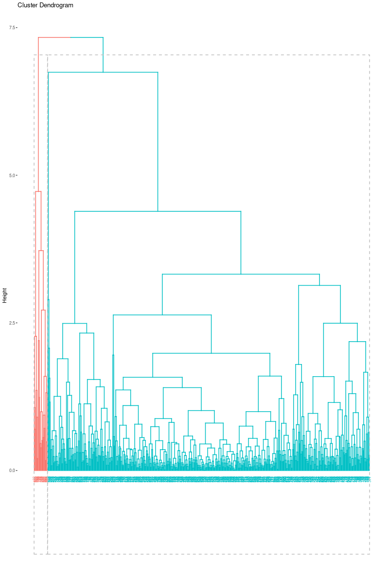
Now, we can again visualize the dendogram. However, this time, we can color the clusters.
fviz_dend(hc_e, # clustering result
          k = 2, # cluster number
          cex = 0.5,
          color_labels_by_k = TRUE,
          rect = TRUE )

Just as we did in the previous clustering algorithms, we can also visualize cluster graph with fviz_cluster function in the factoextra package:
fviz_cluster(list(data = pcadata, cluster = grupward2),
             ellipse.type = "convex",
             repel = TRUE,
             show.clust.cent = FALSE, ggtheme = theme_minimal())

When the cluster graph is analyzed, overlap can be observed. It can be seen that the separation occurs only in both PC1 and PC2. While the variance in the first cluster shown in red is high, the variance in the second cluster shown in green is low.
Average Linkage Method
Average linkage, also known as UPGMA (Unweighted Pair Group Method with Arithmetic Mean), is a hierarchical clustering method that calculates the distance between clusters as the average distance between all pairs of points in the two clusters being merged.
To understand how average linkage works, let’s assume we have n data points and we start with each point in its own cluster. At each step, we merge the two clusters that have the smallest average distance between all pairs of points.
The first step in average linkage is to compute the pairwise distances between all of the data points. This can be done using any distance metric, such as Euclidean distance or Manhattan distance. Next, we compute the average distance between all pairs of points in each cluster. We then merge the two clusters with the smallest average distance, and update the pairwise distances between the new merged cluster and the remaining clusters.
One of the advantages of average linkage is that it tends to produce clusters that are well-separated and roughly equal in size. However, it can also be sensitive to outliers, since it takes the average of all pairwise distances between clusters.
Average Linkage Method in R
Since I covered cophenetic distance in the Ward’s Minimum Variance Method, I will not share it with you in this part. However, I need to state that Euclidean distance again gave the better results. In addition, methods to determine optimal number of clusters, again, suggested 2 as the optimal number of clusters.
Again, you can use fviz_dend function in the factoextra package to visualise dendogram of a hierarchical clustering with the object you created from hierarchical clustering with the function hclust from stats package.
hc_e2 <- hclust(d=dist_euc, method="average")
fviz_dend(hc_e2,cex=.5)
As we can see from the dendogram easily, it is very different from the Ward’s dendogram. It seems clusters are highly unbalanced with respect to the Ward. This may cause a problem for the cluster analysis. However, it is a beneficial example to show that linkage is highly dependent on the data set. It is crucial to decide the best linkage method for the data. One way to decide the linkage is to check the descriptive statistics of the data set to see if there are outliers. Another way is to try all of the linkage methods to see which dendogram looks fine.
Again, it is hard to interpret it from the dendogram, but, we will continue with 2 clusters. One reason is the methods to determine the optimal number of clusters suggested cluster number to be 2. Another reason is to compare the result with Ward’s Minimum Variance methods.
grupav2 <- cutree(hc_e2, k = 2)
grupav2
table(grupav2)
> grupav2
  [1] 1 2 2 2 2 2 2 2 2 2 2 2 1 2 2 2 2 2 2 2 2 2 2 2 2 1 2 2 2 2 2 2 2 2 2 2 2
 [38] 2 2 2 2 2 2 2 2 2 2 2 2 2 2 2 2 2 2 2 2 2 2 2 2 2 2 2 2 2 2 2 2 2 2 2 2 2
 [75] 2 2 2 2 1 2 2 2 1 2 2 2 2 2 2 2 2 2 2 2 2 2 2 2 2 2 2 2 2 2 2 2 2 2 1 2 2
[112] 2 2 2 2 2 2 2 2 2 2 2 1 2 2 2 2 2 2 2 2 2 2 2 2 2 2 2 2 2 2 2 2 2 2 2 2 2
[149] 2 2 2 2 2 2 2 2 2 2 2 2 2 2 2 2 2 2 2 2 2 2 2 2 2 2 2 2 2 2 2 2 1 1 2 2 2
[186] 2 2 2 2 2 2 2 2 2 2 2 2 2 2 2 2 2 1 2 2 2 2 2 2 2 2 2 1 2 2 2 2 2 2 2 2 2
[223] 2 2 2 2 2 2 2 2 2 2 2 2 2 2 2 2 2 2 2 2 2 2 2 2 2 2 2 2 2 2 2 2 2 2 2 1 1
[260] 2 2 2 2 2 2 2 2 2 2 2 2 2 2 2 2 2 2 2 2 2 2 2 2 2 2 2 2 2 2 2 2 2 2 2 2 2
[297] 2 2 2 2 2 2 1 2 2 2 2 2 2 2 2 2 2 2 2 2 2 2 2 2 2 2 2 1 2 2 2 2 2 2 2 2 2
[334] 2 2 2 2 2 2 2 2 2 2 2 2 2 2 2 2 2 2 1 1 2 2 2 2 2 2 2 2 2 2 2 2 2 2 2 2 2
[371] 2 2 2 2 2 2 2 2 2 2 2 2 2 2 2 2 2 2 2 2 2 2 2 1 2 2 2 2 2 2 1 2 2 2 2 2 2
[408] 2 2 2 2 2 2 2 2 2 2 2 2 2 2 2 2 2 2 2 2 2 2 2 2 2 2 2 2 2 2 2 2 2 2 2 2 2
[445] 2 2 2 2 2 2 2 2 2 2 2 2 2 2 2 2 2 1 2 2 2 2 2 2 2 2 2 2 2 2 2 2 2 2 2 2 2
[482] 2 2 2 2 2 2 2 2 2 2 2 2 2 2 2 2 2 2 2 2 2 2 2 2 2 2 2 2 2 2 2 2 2 2 2 2 2
[519] 2 2 2 1 2 2 2 2 2 2 2 2 2 2 2 2 2 2 2 2 2 2 2 2 2 2 2 2 2 2 2 2 2 2 2 2 2
[556] 2 2 2 2 2 2 2 2 1 2 2 2 1 2
> table(grupav2)
grupav2
  1   2
 23 546
As we can see from the output, clusters are highly unbalanced. This output was expected since we observe dendogram.
Again, we can again visualize the dendogram. However, this time, we can color the clusters.
fviz_dend(hc_e2, k = 2,
          cex = 0.5,
          color_labels_by_k = TRUE,
          rect = TRUE )
Again, just as we did in the previous clustering algorithms, we can also visualize cluster graph with fviz_cluster function in the factoextra package:
fviz_cluster(list(data = pcadata, cluster = grupav2),
             ellipse.type = "convex",
             repel = TRUE,
             show.clust.cent = FALSE, ggtheme = theme_minimal())

That was the end of this post. Just like always:
“In case I don’t see ya, good afternoon, good evening, and good night!”
References
[1] Ward Jr, J. H. (1963). Hierarchical grouping to optimize an objective function. Journal of the American statistical association, 58(301), 236–244.
[2] Roux, M. (2015). A comparative study of divisive hierarchical clustering algorithms. arXiv preprint arXiv:1506.08977.
[3] Kassambara, Alboukadel. Practical guide to cluster analysis in R: Unsupervised machine learning. Vol. 1. Sthda, 2017.
[4] Kassambara, Alboukadel. Practical guide to cluster analysis in R: Unsupervised machine learning. Vol. 1. Sthda, 2017.
[5] Kassambara, Alboukadel. Practical guide to cluster analysis in R: Unsupervised machine learning. Vol. 1. Sthda, 2017.
[6] Kassambara, Alboukadel. Practical guide to cluster analysis in R: Unsupervised machine learning. Vol. 1. Sthda, 2017.
[7] Ward Jr, J. H. (1963). Hierarchical grouping to optimize an objective function. Journal of the American statistical association, 58(301), 236–244.
[8] Triayudi, A., & Fitri, I. (2018). Comparison of parameter-free agglomerative hierarchical clustering methods. ICIC Express Letters, 12(10), 973–980.