In the second post of the unsupervised statistical learning in R series, I will share with you the k-means clustering algorithm. I believe, at first, it is beneficial to define what clustering is, before explaining k-means clustering. Clustering can be defined as partitioning observation in a data set according to their similarity. We expect that observations in the same cluster to be similar as much as possible. Conversely, observations in the different clusters need to be dissimilar. What do we mean by this similarity? Similarity in the clustering algorithms are calculating as distance. Observations which are closest to each other are considered as the similar observations. There are more than 30 metrics that can bu used to calculate distance between two points. However, Euclidean and Manhattan distance are the most widely used distance metrics.
What is k-means?
The center of each cluster, or centroid, in k-means clustering corresponds to the mean of the points allocated to the cluster. The fundamental principle of k-means clustering is to define clusters with the goal of minimizing total intra-cluster variation, also referred to as total within-cluster variation. Various k-means algorithms are available. The common approach is the Hartigan-Wong algorithm (1979), which sums the squared distances between items and the matching centroid to determine the total within-cluster variation[1],[2],[3]. The most crucial point in k-means is to decide the cluster number k. There are lots of methods to determine optimum number of cluster, however, you can see the most common ones in here.
Mathematical formula of the k-means is as follows:
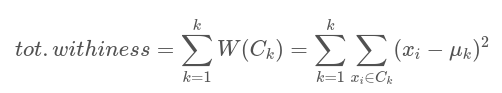
where:
-
xi is a data point belonging to the cluster Ck
-
μk is the mean value of the points assigned to the cluster Ck
Step by Step
The steps to perform k-means clustering are:
Step 1:
Select k, the number of clusters, that you want to form in the data. As I mentioned before, there are lots of methods to determine the optimal number of clusters. You can see the first postof this series for detailed information about optimal cluster number determination.
Step 2:
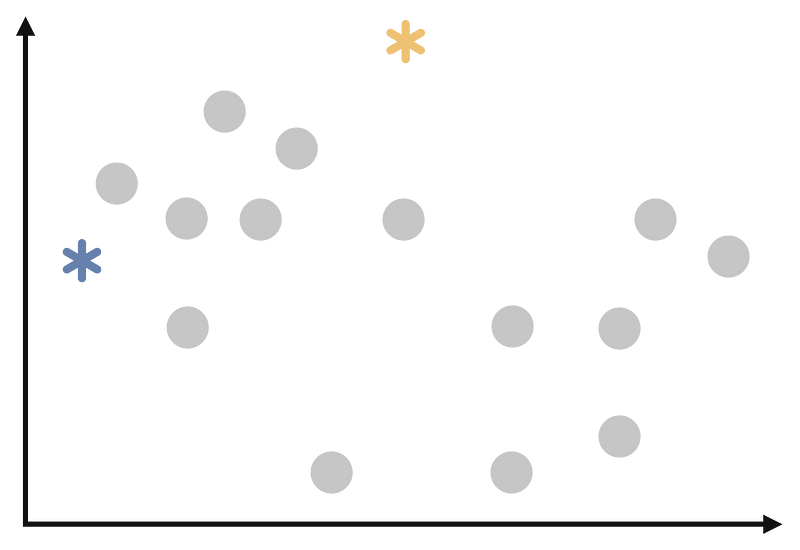
Select k random points from the dataset as the initial centroids (cluster center).
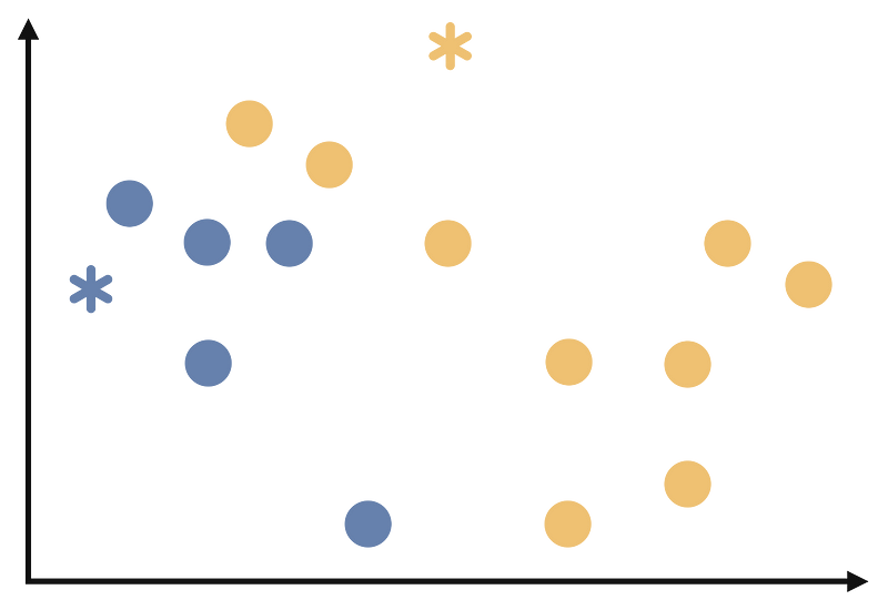
As first assume we have a data like the follows:
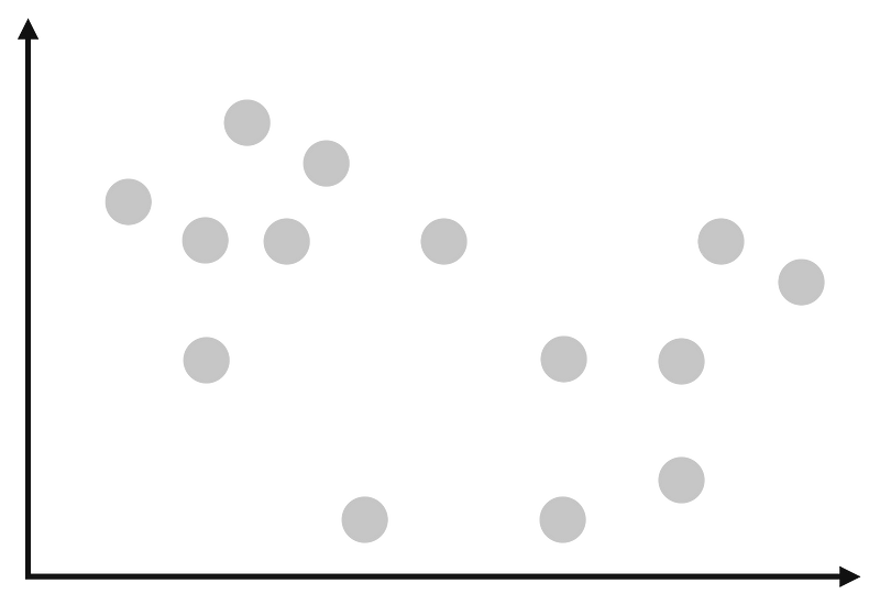
We need to select a random points to be cluster center. This will look like the following:
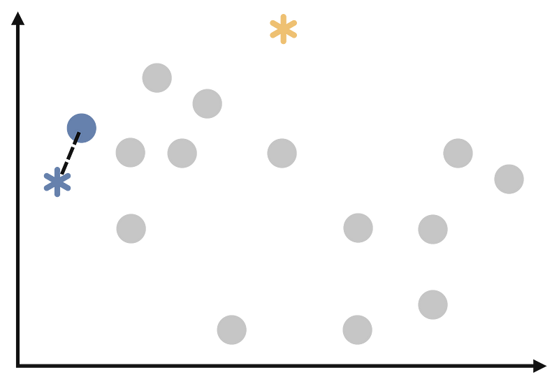
Step 3:
Assign each observation to the cluster whose centroid is closest to it. We will start to assign each point as follows.
At the end of this step, our process will look like the follows.
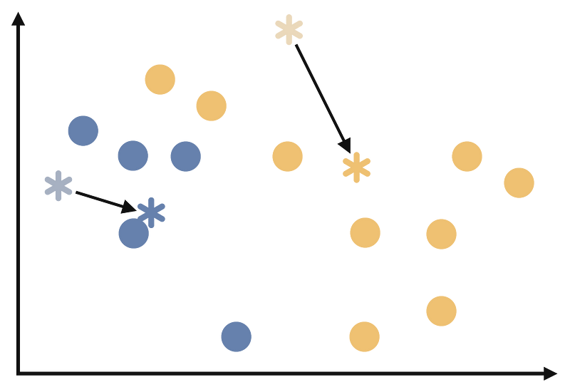
Step 4:
Recalculate the centroids as the mean of all the observations in each cluster. Consider the last step. All of the points in the data is clustered. At this step, we are calculating the new centroids as follows.
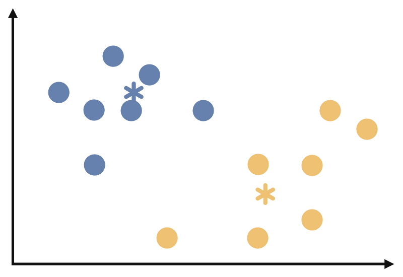
Step 5:
Repeat steps 3 and 4 until the cluster assignments no longer change or reach a maximum number of iterations. At the end of these iterations our clustering will look like the follows:
Data Preparation for k-means
In general, the data preparation for a cluster analysis in unsupervised learning should go as follows:
-
Missing values in the data should be eliminated/estimated.
-
To make variables comparable, the data must be scaled or normalized. The process of standardization entails altering the variables so that their means are 0 and standard deviations are 1.[4]
-
PCA can help to enhance the performance of a clustering algorithm by transforming the data into a new coordinate system that better separates the underlying clusters. This can lead to more accurate and meaningful results, especially for datasets with complex structures. [5]
-
PCA can be used to reduce the number of features in a high-dimensional dataset, which can help improve the performance of a clustering algorithm. By reducing the dimensionality, PCA can also help to reduce noise and eliminate multicollinearity in the data, making it easier to interpret the results of a clustering analysis.[6]
k-means in R
There are many packages and functions available to implement the k-means algorithm in R. In this article, I will show you the kmeans function in the statspackage and the eclustfunction in the factoextrapackage. I will use Breast Cancer Wisconsin dataset from the UCI Machine Learning Repository.
The dataset contains information about tumor cells. The task in this project was to extract the variable containing the information labeled as benign or malignant from the dataset and cluster the tumors as benign or malignant using clustering algorithms. There are 569 observations and 32 variables in the dataset. However, some variables are mean of the other variables. Thus, these variables are removed from the dataset. Moreover, ID and variable about class information is also removed. Given the high correlation between pairs of variables and the high dimensionality, I applied PCA to the dataset. I have not included this step as it is not the subject of this paper.
If you read the first post, you will remember that I compared cluster number determination methods on the same dataset. All methods predominantly suggested two cluster numbers. That is why I will cluster the data for 2 clusters.
We do clustering with the kmeansfunction and then we store the clustering result in the km_dataobject. Then we print this object with the printfunction.
km_data <- kmeans(df, # data to cluster
                  2, # k, cluster number
                  nstart=25 # number of iteration
                  )
print(km_data)
K-means clustering with 2 clusters of sizes 398, 171

Cluster means:
        PC1         PC2
1  1.289695 -0.03214799
2 -3.001746  0.07482399

Clustering vector:
  [1] 2 2 2 2 2 2 2 2 2 2 1 2 2 1 2 2 1 2 2 1 1 1 2 2 2 2 2 2 2 2 2 1 2 2 2 2 1 1 1 1 1 1 2 1 1 2 1 1 1 1 1 1 1 2 1 1 2 2 1 1 1 1 2 1 1 2 1 1
 [69] 1 1 2 1 2 1 1 1 1 2 2 1 1 1 2 2 1 2 1 2 1 2 1 1 1 1 2 2 1 1 1 1 1 1 1 1 1 2 1 1 2 1 1 1 2 1 1 1 1 2 2 1 1 2 2 1 1 1 1 2 2 2 1 2 2 1 2 1
[137] 1 1 2 1 1 1 1 1 1 1 2 1 1 1 1 1 2 1 1 1 2 1 1 1 1 2 2 1 2 1 1 1 2 1 1 1 2 1 1 1 1 2 1 1 2 2 1 1 1 1 1 1 1 1 2 1 1 1 2 1 2 2 2 1 1 2 2 2
[205] 1 1 1 1 1 1 2 1 2 2 2 1 1 1 2 2 1 1 1 2 1 1 1 1 1 2 2 1 1 2 1 1 2 2 1 2 1 1 1 1 2 1 1 1 1 1 2 1 2 2 2 1 2 2 2 2 2 1 2 1 2 2 1 1 1 1 1 1
[273] 2 1 1 1 1 1 1 1 2 1 2 2 1 1 1 1 1 1 1 1 1 1 1 1 1 1 1 1 2 1 2 1 1 1 1 1 1 1 1 1 1 1 1 1 1 2 1 1 1 2 1 2 1 1 1 1 2 2 2 1 1 1 1 2 1 2 1 2
[341] 1 1 1 2 1 1 1 1 1 1 1 2 2 1 1 1 1 1 1 1 1 1 1 1 1 2 2 1 2 2 2 1 2 2 1 2 1 1 1 2 1 1 1 1 1 1 1 1 1 2 1 1 2 2 1 1 1 1 1 1 2 1 1 1 1 1 1 1
[409] 2 1 1 1 1 1 1 1 1 2 1 1 1 2 1 1 1 1 1 1 1 1 2 1 2 2 1 1 1 1 1 1 1 2 1 1 2 1 2 1 1 2 1 2 1 1 1 1 1 1 1 1 2 2 1 1 1 1 1 1 2 1 1 1 1 1 1 1
[477] 1 1 1 2 1 1 1 1 1 1 1 2 1 1 1 1 2 1 1 1 1 1 2 2 1 2 1 2 2 1 1 1 1 2 1 1 2 1 1 1 2 2 1 1 1 2 1 1 1 1 1 1 1 1 1 1 1 2 1 2 1 1 1 1 1 1 1 1
[545] 1 1 1 1 1 1 1 1 1 1 1 1 1 1 1 1 1 1 2 2 2 2 1 2 1

Within cluster sum of squares by cluster:
[1] 1121.768 1216.540
 (between_SS / total_SS =  48.5 %)
When we examine the output, we first see how many elements there are for each cluster. It is noticed that there are 398 observations in the first cluster and 171 observations in the second cluster. It is possible to say that this is unbalanced. Then the cluster means section appears. In this section, we see the values taken by the centroids of each cluster. Since k-means takes the centroids as the mean of the cluster, it would not be wrong to say that we see the means of the clusters. In the clustering vector section, we see to which cluster each observation in the dataset is assigned. Each clustering algorithm assigns cluster names as 1,2,3…. The last section shows the within cluster sum of squares values for each cluster. This is an important value for the explanatory power of clustering. We want it to be as high as possible.
Of course, it is quite possible to make a more detailed comment on this output. But this is not our only option. We can visualize the clustering result with the fviz_cluster function in the factoextra package. Since the factoextra package uses the ggplot2 package for all visualizations, you can make the same changes to the ggplot2 plots that you can make to the graphs you plot with the fviz_cluster function.
library(factoextra)
fviz_cluster(km_data,# clustering result
             data = pcadata, # data
             ellipse.type = "convex",
             star.plot = TRUE,
             repel = TRUE,
             ggtheme = theme_minimal()
)

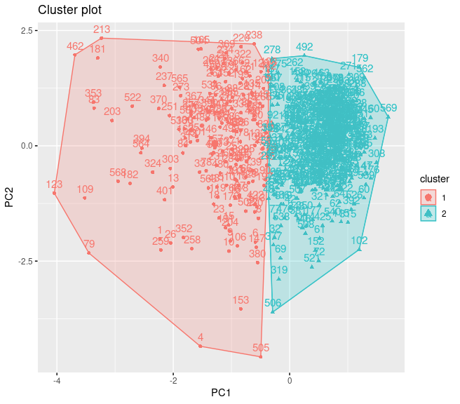
It may be possible to interpret this plot as follows:
-
Separation can be observed only in PC1 dimension.
-
Within sum of square of the cluster 2 is much than the cluster 1.
-
The reason of this needs to be the difference between observation numbers of the clusters.
-
There is no visible overlap between clusters.
It is also possible to cluster data with eclustfunction from factoextra package.
k2m_data <- factoextra::eclust(df, # data
                               "kmeans", # clustering algorithm
                               k = 2, # cluster number
                               nstart = 25, # iteration number
                               graph = F)
k2m_data
K-means clustering with 2 clusters of sizes 171, 398

Cluster means:
        PC1         PC2
1 -3.001746  0.07482399
2  1.289695 -0.03214799

Clustering vector:
  [1] 1 1 1 1 1 1 1 1 1 1 2 1 1 2 1 1 2 1 1 2 2 2 1 1 1 1 1 1 1 1 1 2 1 1 1 1 2 2 2 2 2 2 1 2 2 1 2 2 2 2 2 2 2 1 2 2 1 1 2 2 2 2 1 2 2 1 2 2
 [69] 2 2 1 2 1 2 2 2 2 1 1 2 2 2 1 1 2 1 2 1 2 1 2 2 2 2 1 1 2 2 2 2 2 2 2 2 2 1 2 2 1 2 2 2 1 2 2 2 2 1 1 2 2 1 1 2 2 2 2 1 1 1 2 1 1 2 1 2
[137] 2 2 1 2 2 2 2 2 2 2 1 2 2 2 2 2 1 2 2 2 1 2 2 2 2 1 1 2 1 2 2 2 1 2 2 2 1 2 2 2 2 1 2 2 1 1 2 2 2 2 2 2 2 2 1 2 2 2 1 2 1 1 1 2 2 1 1 1
[205] 2 2 2 2 2 2 1 2 1 1 1 2 2 2 1 1 2 2 2 1 2 2 2 2 2 1 1 2 2 1 2 2 1 1 2 1 2 2 2 2 1 2 2 2 2 2 1 2 1 1 1 2 1 1 1 1 1 2 1 2 1 1 2 2 2 2 2 2
[273] 1 2 2 2 2 2 2 2 1 2 1 1 2 2 2 2 2 2 2 2 2 2 2 2 2 2 2 2 1 2 1 2 2 2 2 2 2 2 2 2 2 2 2 2 2 1 2 2 2 1 2 1 2 2 2 2 1 1 1 2 2 2 2 1 2 1 2 1
[341] 2 2 2 1 2 2 2 2 2 2 2 1 1 2 2 2 2 2 2 2 2 2 2 2 2 1 1 2 1 1 1 2 1 1 2 1 2 2 2 1 2 2 2 2 2 2 2 2 2 1 2 2 1 1 2 2 2 2 2 2 1 2 2 2 2 2 2 2
[409] 1 2 2 2 2 2 2 2 2 1 2 2 2 1 2 2 2 2 2 2 2 2 1 2 1 1 2 2 2 2 2 2 2 1 2 2 1 2 1 2 2 1 2 1 2 2 2 2 2 2 2 2 1 1 2 2 2 2 2 2 1 2 2 2 2 2 2 2
[477] 2 2 2 1 2 2 2 2 2 2 2 1 2 2 2 2 1 2 2 2 2 2 1 1 2 1 2 1 1 2 2 2 2 1 2 2 1 2 2 2 1 1 2 2 2 1 2 2 2 2 2 2 2 2 2 2 2 1 2 1 2 2 2 2 2 2 2 2
[545] 2 2 2 2 2 2 2 2 2 2 2 2 2 2 2 2 2 2 1 1 1 1 2 1 2

Within cluster sum of squares by cluster:
[1] 1216.540 1121.768
 (between_SS / total_SS =  48.5 %)

Available components:

 [1] "cluster"      "centers"      "totss"        "withinss"     "tot.withinss" "betweenss"    "size"         "iter"         "ifault"
[10] "clust_plot"   "silinfo"      "nbclust"      "data"
If you examine the output of the k2m_data object, you can see that it gives almost the same output as the kmeans function. There will be other information that you can get from the clustering done with the eclustfunction. For example, with k2m_data$silinfo you can get the silhouette values for each observation. This can help you to question the validity of your clustering. In addition, you can also plot the clustering plot without the need for the fviz_cluster function. There are two ways to do this.
At first you can change graph argument in the function as follows:
k2m_data <- factoextra::eclust(pcadata,
                               "kmeans",
                               k = 2,
                               nstart = 25,
                               graph = T)
You can also reach the plot with the following code:
k2m_data$clust_plot
At the end, you will have a plot like the follows:
Just like always:
“In case I don’t see ya, good afternoon, good evening, and good night!”
References
[1] Hartigan, John A., Manchek A. Wong. Algorithm AS 136: A k-means clustering algorithm. Journal of the royal statistical society. series c (applied statistics) 28., 100–108, 1979
[2] Kassambara, Alboukadel. Practical guide to cluster analysis in R: Unsupervised machine learning. Vol. 1. Sthda, 2017.
[3] James, G., Witten, D., Hastie, T., & Tibshirani, R. (2013). An introduction to statistical learning (Vol. 112, p. 18). New York: springer.
[4] Kassambara, Alboukadel. Practical guide to cluster analysis in R: Unsupervised machine learning. Vol. 1. Sthda, 2017.
[5] Ben-Hur, Asa, and Isabelle Guyon. Detecting stable clusters using principal component analysis. Functional genomics. Humana press, 159–182, 2003.
[6] Ding, Chris, and Xiaofeng He. K-means clustering via principal component analysis. Proceedings of the twenty-first international conference on Machine learning. 2004.