In the previous post of this series, I covered how k-means clustering works in detail. In this post, I will try to explain the k-medoids algorithm, also known as Partitioning Around Medoids. First, I will explain what k-medoids is, then I will explain how it works step by step, and then I will explain how to implement it using the R program language.
What is k-medoids?
k-medoids is a clustering algorithm that is similar to k-means, but instead of using the mean of the observations in each cluster as the centroid, it uses one of the observations in the cluster as the “medoid.” The main idea behind k-medoids is to define clusters where the total dissimilarity between observations and the medoid is minimized. The k-medoids algorithm is also known as Partitioning Around Medoids (PAM) algorithm.[1], [2]
Step by Step
The steps to perform k-medoids clustering are:
Step 1
Select k, the number of clusters, that you want to form in the data. As I mentioned before, k-medoids and k-means are very similar algorithms. One similarity emerges in this regard. In the first post of this series, I shared a detailed analysis of this step. Although that analysis was based on k-means, you can run it for k-medoids by simply changing the clustering algorithm to k-medoids (pam in R).
Step 2
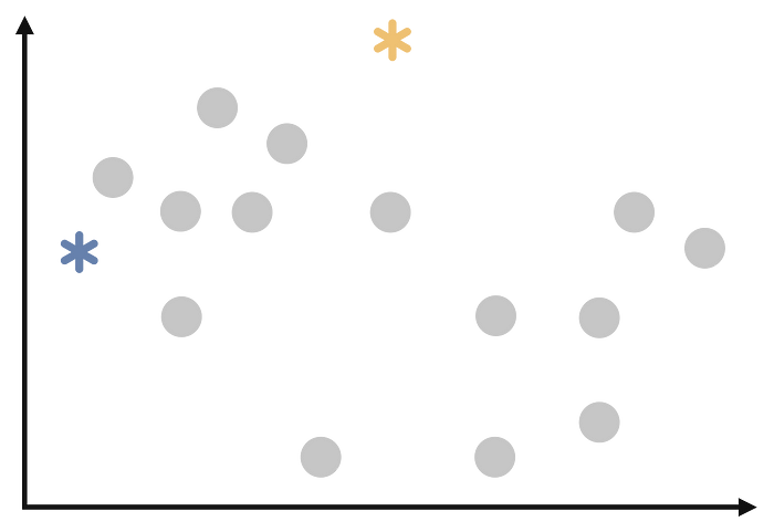
Select k random observations from the dataset as the initial medoids. This is another similarity with k-means. Thus, I will use the same illustration.
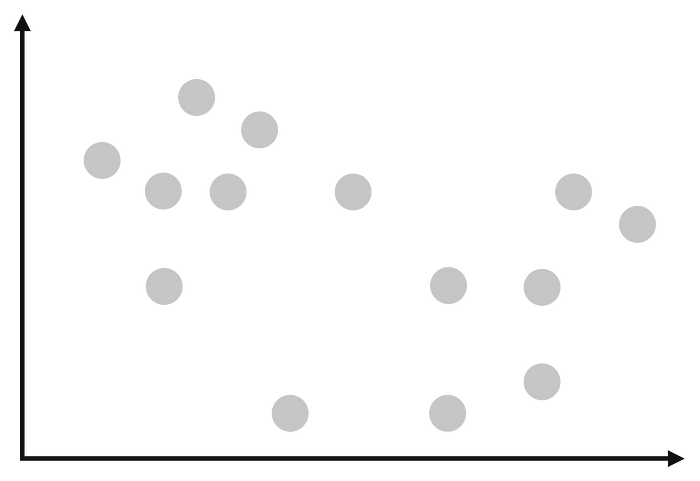
At first, we have a data like the following:
After the second step, we have the following:
Step 3
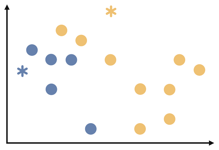
Assign each observation to the cluster whose medoid is closest to it based on a distance metric. This is again the same as k-means. After the third step we will have the following:
Step 4
Recalculate the medoids as the observation in each cluster that minimizes the total dissimilarity to the other observations in the same cluster. This is where the difference between k-means and k-medoids occurs. As I mentioned in the previous post, in the k-means algorithm we are ecalculating the centroids as the mean of all the observations in each cluster. But when it comes to k-medoids, we are recalculate the medoids as the observation in each cluster that minimizes the total dissimilarity to the other observations in the same cluster.
Step 5
Repeat steps 3 and 4 until the cluster assignments no longer change or reach a maximum number of iterations.
The gif below repeats all the steps of k-medoids. I included it in the article because I thought it might be useful for understanding the algorithm.

It’s important to note that k-medoids is more robust to noise and outliers than k-means, it’s also more efficient for handling categorical variables. However, k-medoids is more computationally expensive than k-means because it requires the calculation of all pairwise distances between observations at each iteration. Like k-means, k-medoids is sensitive to the initial conditions and it’s recommended to run the algorithm multiple times and choose the best solution.
k-medoids in R
There are many packages and functions available to implement the k-means algorithm in R. In this article, I will show you the pam function in the clusterpackage. I will use Breast Cancer Wisconsin dataset from the UCI Machine Learning Repository.
The dataset contains information about tumor cells. The task in this project was to extract the variable containing the information labeled as benign or malignant from the dataset and cluster the tumors as benign or malignant using clustering algorithms. There are 569 observations and 32 variables in the dataset. However, some variables are mean of the other variables. Thus, these variables are removed from the dataset. Moreover, ID and variable about class information is also removed. Given the high correlation between pairs of variables and the high dimensionality, I applied PCA to the dataset. I have not included this step as it is not the subject of this paper.
If you read the first post, you will remember that I compared cluster number determination methods on the same dataset. All methods predominantly suggested two cluster numbers. That is why I will cluster the data for 2 clusters.
We do clustering with the pamfunction and then we store the clustering result in the pam_dataobject. Then we print this object with the printfunction.
pam_data <- pam(df,2)
print(pam_data)
> print(pam_data)
Medoids:
      ID       PC1        PC2
[1,] 499 -2.357211 0.30131315
[2,] 269  1.358672 0.03762238
Clustering vector:
  [1] 1 1 1 1 1 1 1 1 1 1 2 1 1 1 1 1 2 1 1 2 2 2 1 1 1 1 1 1 1 1 1 2 1 1 1 1 2 2 2 2 2 2 1 2 2 1 2 1 2 2 2 2 2 1 2 2 1 1 2 2 2 2 1 2 2 1 2 2
 [69] 2 2 1 2 1 2 2 1 2 1 1 2 2 1 1 1 2 1 2 1 2 1 2 1 2 2 1 1 2 2 2 2 2 2 2 2 2 1 2 2 1 2 2 2 1 2 2 2 2 1 1 1 2 1 1 2 2 2 2 1 1 1 2 1 1 2 1 2
[137] 2 2 1 2 2 1 2 2 2 2 1 2 2 2 2 2 1 2 2 2 1 2 2 2 2 1 1 2 1 2 2 1 1 2 2 2 1 2 2 2 2 1 2 2 1 1 2 2 2 2 1 2 2 2 1 2 2 2 1 2 1 1 1 1 2 1 1 1
[205] 2 2 2 1 2 2 1 2 1 1 1 1 2 2 1 1 2 2 2 1 2 2 2 2 2 1 1 2 2 1 2 2 1 1 2 1 2 2 2 2 1 2 2 2 2 2 1 2 1 1 1 2 1 1 1 1 1 2 1 2 1 1 2 2 2 2 2 2
[273] 1 2 1 2 2 1 2 2 1 2 1 1 2 2 2 2 2 2 1 2 2 2 2 2 2 2 2 2 1 2 1 2 2 2 2 2 2 2 2 2 2 2 2 2 2 1 2 2 2 1 2 1 2 2 2 2 1 1 1 2 2 2 2 1 2 1 2 1
[341] 2 2 2 1 2 2 2 2 2 2 2 1 1 1 2 2 2 2 2 2 2 2 2 2 2 1 1 2 1 1 1 2 1 1 2 1 2 2 2 1 2 2 2 2 2 2 2 2 2 1 2 2 1 1 2 2 2 2 2 2 1 2 2 2 2 2 2 2
[409] 1 2 2 2 2 2 2 2 2 1 2 2 2 1 2 2 2 2 2 2 2 2 1 2 1 1 2 2 2 2 2 2 2 1 2 2 1 2 1 2 2 1 2 1 2 2 2 2 2 2 2 2 1 1 2 2 2 2 2 2 1 2 2 2 2 2 2 2
[477] 2 2 2 1 2 2 2 2 1 2 2 1 2 2 2 2 1 2 2 2 2 2 1 1 2 1 2 1 1 2 2 2 2 1 2 2 1 2 2 2 1 1 2 2 2 1 2 2 2 2 2 2 2 2 2 2 2 1 2 1 1 2 2 2 2 2 2 2
[545] 2 2 2 2 2 2 2 2 2 2 2 2 2 2 2 2 2 2 1 1 1 1 1 1 2
Objective function:
   build     swap
1.806580 1.700399

Available components:
 [1] "medoids"    "id.med"     "clustering" "objective"  "isolation"  "clusinfo"   "silinfo"    "diss"       "call"       "data"
If we examine the output obtained with the print function; at first we can access the medoid information of each cluster for both PC1 and PC2 dimensions. In addition, we can also see how many observations are in each cluster. As a result of this analysis, there are 499 observations in the first cluster and 269 elements in the second cluster. The medoid of the first cluster is (-2.357211, 0.30131315). The second cluster’s medoid is (1.358672, 0.03762238). Then we see the clustering vector, which contains the information to which cluster each observation is assigned. Finally, we see the objective function. build represents the first step that I explained in the step-by-step calculation section and swap represents the third step.
Of course, it is quite possible to make a more detailed comment on this output. But this is not our only option. We can visualize the clustering result with the fviz_cluster function in the factoextra package. Since the factoextra package uses the ggplot2 package for all visualizations, you can make the same changes to the ggplot2 plots that you can make to the graphs you plot with the fviz_cluster function.
fviz_cluster(df, # data
             ellipse.type = "convex", # type of the clusters' appearence
             repel = T,
             ggtheme = theme_classic()
)
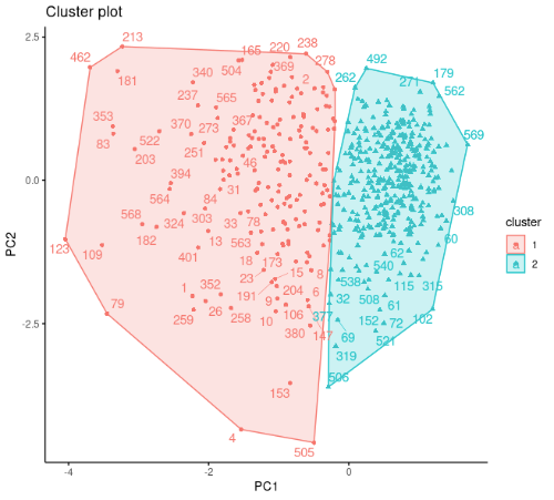
According to the cluster plot, no overlap is observed .The separation occurs only in the PC1 dimension. The variance in the first cluster shown in red color is higher.
Just like always:
“In case I don’t see ya, good afternoon, good evening, and good night!”
References
[1] Kaufman, L., & Rousseeuw, P. (1987). Clustering by means of medoids. Statistical Data Analysis Based on the L1-Norm and Related Methods, Y. Dodge Ed.
[2] Kaufman, L., & Rousseeuw, P. J. (2009). Finding groups in data: an introduction to cluster analysis. John Wiley & Sons.