I plan to write many series of articles in my medium journey that I started with data visualization. In addition to series such as Unsupervised Statistical Learning, Supervised Statistical Learning, Math for Data Science, Statistics and Probability, I will also touch on the intersection of my undergraduate degree in philosophy and data science. In this way, I think I can support analytical and critical thinking for the individual who is on a data science journey. I will also have some articles that I plan to combine culture and data science.
In this regard, I am with you with the first post of the first series, Unsupervised Statistical Learning. In this post, I will talk about the methods to determine the optimal number of clusters. In this post, as in every other post, I will talk about what methods mean, what they are used for and how to do it step by step. I will run all methods in R by using the k-means clustering algorithm and always use the same dataset (Breast Cancer Wisconsin).
Why do we need to determine cluster number?
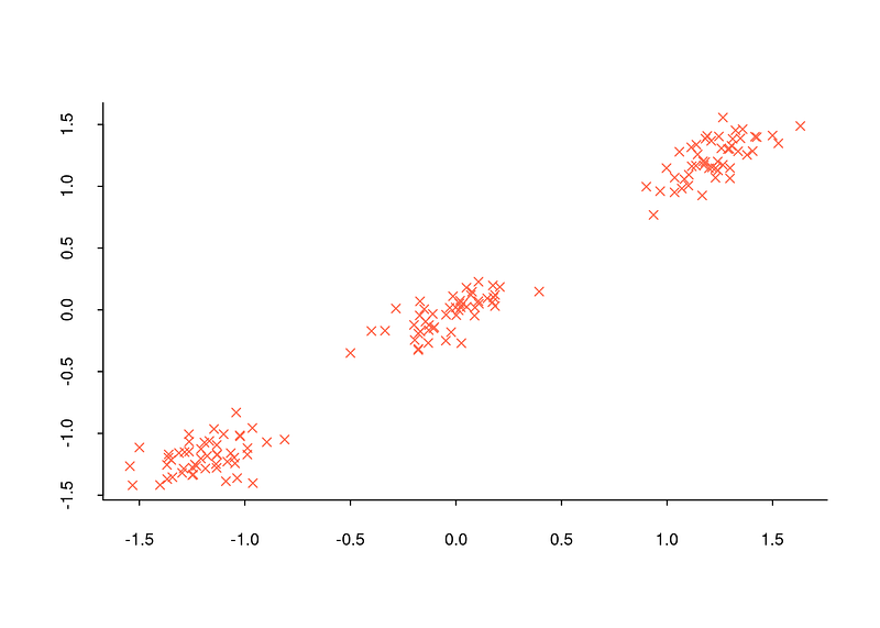
The first reason is that the number of clusters must be predetermined for the clustering algorithms to work. For example, many algorithms such as k-means, k-medoids, hierarchical clustering need to know the number of clusters in order to work. Depending on the data set and the work done with that data set, we may know the number of clusters in advance. For example, in the plot below, it is quite possible to determine the number of clusters with a scatter plot.
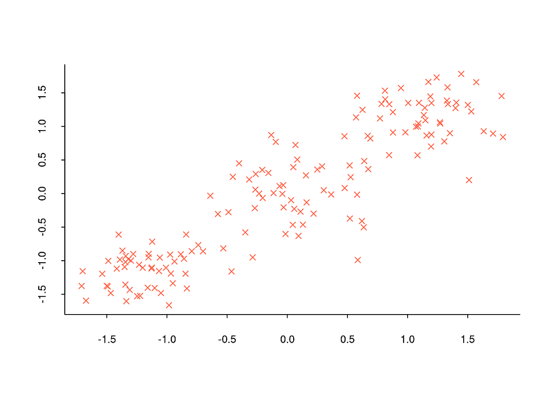
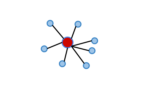
However, determining the number of clusters in commonly encountered data sets is too complex to be achieved simply by observing the overall structure of the data set with a scatter plot. For example, when the scatter plot below is analyzed, it is not possible to tell how many clusters the data set is divided into.
However, since situations like the one in the above plot are frequently encountered, some methods have been proposed to determine the number of clusters. I will now explain what some of these methods are, how they are calculated step by step and their implementation in R.
Elbow Method
The elbow method, also known as total within sum of squares, is a technique used to determine the optimal number of clusters for a k-means clustering analysis. The idea behind the elbow method is to run k-means clustering on the dataset for a range of values of k (number of clusters), and for each value of k calculate the sum of squared distances of each point from its closest centroid (SSE). The elbow point is the point on the plot of SSE against the number of clusters (k) where the change in SSE begins to level off, indicating that adding more clusters doesn't improve the model much. [1], [2]
The steps to perform the elbow method are:
-
Select a range of k values, usually from 1 to 10 or the square root of the number of observations in the dataset.
-
Run k-means clustering for each k value and calculate the SSE (sum of squared distances of each point from its closest centroid).
-
Plot the SSE for each k value.
-
The point on the plot where the SSE starts to decrease at a slower rate is the elbow point, and the corresponding number of clusters is the optimal value for k.
Undoubtedly, the Elbow method is one of the most widely used methods. It can be said to be a method that follows the same logic as k-means. However, it would not be correct to say that it gives good results under all circumstances. Sometimes it can even be said to be misleading. For this reason, although I use the elbow method in every cluster analysis, I do not rely on it alone.
In R, factoextra packages offers fancy plots for some of the methods to determine optimal number of clusters in this post. I will use fviz_nbclust function to visualize elbow method for the dataset.
fviz_nbclust(df, # data
             kmeans, # clustering algorithm
             nstart = 25, # if centers is a number, how many random sets should be chosen?(default is 25)
             iter.max = 200, # the maximum number of iterations allowed.
             method = "wss") # elbow method
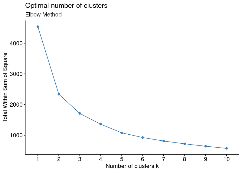
For example, the output above shows that there is no sharp elbow. For this reason, it draws attention as a result open to interpretation. An interpretation based on this elbow may therefore lead to incorrect results.
Average Silhouette Method
Average silhouette method measures how well-defined a particular cluster is, and how well-separated it is from other clusters. At this point, it is necessary to state that Silhouette value is calculated for each observation in the data set. Average of the silhouette value of all observations gives us the average silhouette value, which is the silhouette value of the clustering analysis [3] , [4].
The steps to calculate silhouette value for a observation are:
-
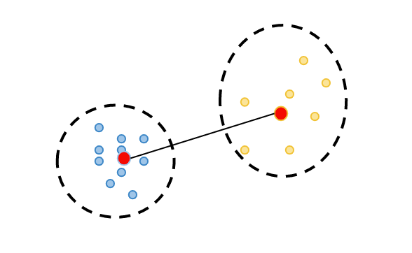
calculate cluster tightness: the average distance purple observation to all blue observations which all are in the same cluster, which is called a(i).
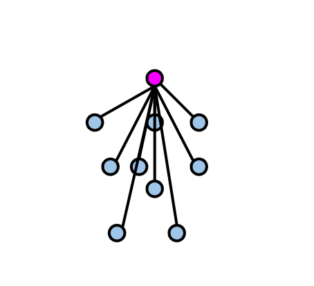
2. calculate cluster separation: observation's minimum distance to all the observations in a different cluster(yellow cluster), which is called b(i).
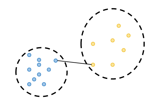
3. calculate silhouette coefficient: calculate its silhouette value "s(i)" as the difference between the b(i) and a(i), divided by the maximum of these two distances:

After calculating silhouette coefficient of each observation, we can finally, calculate the average silhouette value for all observations: mean(si). To determine the number of clusters, we usually cluster each number of clusters for a range of 2 to 10 clusters and obtain the average silhouette value for each number of clusters. The silhouette value ranges from -1 to 1, where a value of 1 indicates a strong similarity to the other observations in its own cluster, and a value of -1 indicates a strong similarity to observations in another cluster. In other words, the number of clusters with the highest silhouette value is the number of clusters we will determine.
Again fviz_nbclust function is a way to see average silhoutte plot to decide the optimal number of clusters:
fviz_nbclust(df, # data
             kmeans, # clustering algorithm
             method = "silhouette") # silhouette
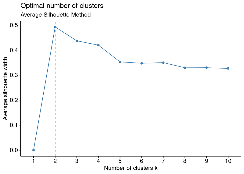
As can be easily seen from the plot, the clustering model with the highest silhouette value is the clustering for 2 clusters. Therefore, it can be inferred that the optimal number of clusters is two. However, when the silhouette values on the y-axis are examined, the silhouette value for the number of clusters 3 is also quite close, although the number of clusters 2 is the highest. For this reason, it would be more useful to always run the clustering algorithm for both 2 and 3 clusters and interpret the results.
Gap Statistic Method
Gap Statistic Method compares the observed within-cluster variation for different values of k with the variation expected under a null reference distribution of the data. [5]
The steps to perform the gap statistic method are:
-
Select a range of k values, usually from 1 to 10 or the square root of the number of observations in the dataset.
-
Run the clustering algorithm (such as k-means or hierarchical clustering) for each k value and calculate the within-cluster variation Wk.
-
Generate B reference datasets by randomly sampling the original data and calculate the within-cluster variation W*k for each dataset.
-
Calculate the gap statistic
-
Plot the gap statistic for each k value.
-
The k value that corresponds to the maximum gap statistic is the optimal number of clusters.
Again fviz_nbclust function is a way to see gap statistic plot to decide the optimal number of clusters:
fviz_nbclust(df,
             kmeans ,
             nstart = 25,
             method = "gap_stat")
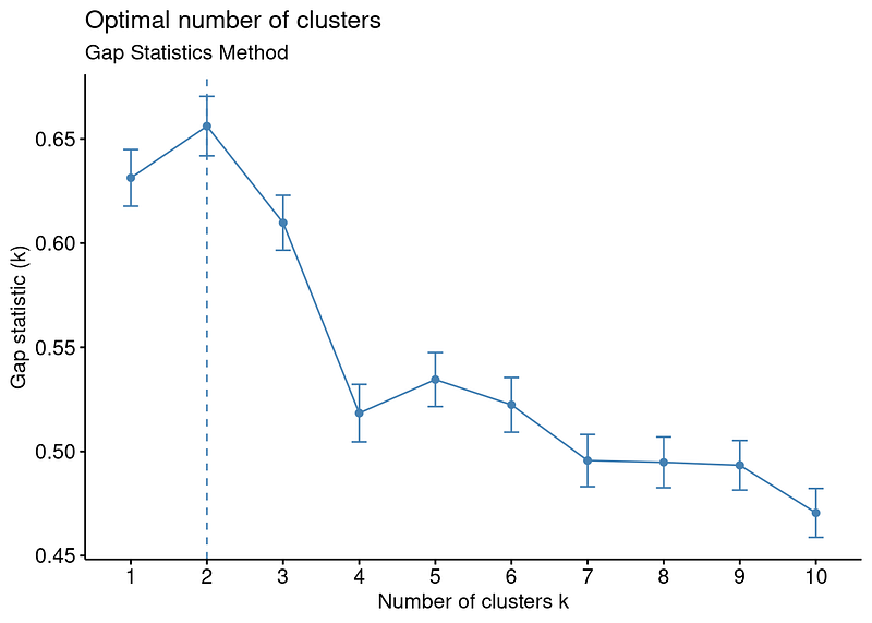
Just like Average Silhouette Method, Gap Statistic Method is also offers 2 as the optimal number of clusters.
Calinski — Harabasz Method
The Calinski-Harabasz index (also known as the Variance Ratio Criterion) is a commonly used evaluation metric for comparing different clustering solutions in unsupervised learning. It is a ratio of the between-cluster variance and the within-cluster variance, and it is used to determine the number of clusters that should be used in a clustering solution[6].
The steps to perform the calinski-harabasz method are:
-
calculate within cluster sum of squares (WCSS): the sum of the squared distances between each observation and its corresponding cluster center(barycenter).
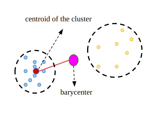
2. calculate between cluster sum of squares (BCSS): calculate the sum of the squared distances between each cluster center and the overall mean of all the observation.
3. (BCSS / WCSS) — (n-k) / (k-1)
where,
k: total cluster number,
n:total observation number
The Calinski-Harabasz index ranges from 0 to infinity, with a higher value indicating a better clustering.
For the Calinski — Harabasz method, there is no visualization function in R as in the methods I mentioned before. For this reason, I will write a function that calculates and visualizes the Calinski — Harabasz values for the clusters 2 to 10 using the calinhara function in the fpc package.
library(fpc) # for calinhara function

fviz_ch <- function(data) {
  ch <- c()
  for (i in 2:10) {
    km <- kmeans(data, i) # perform clustering
    ch[i] <- calinhara(data, # data
                       km$cluster, # cluster assignments
                       cn=max(km$cluster) # total cluster number
                       )
  }
  ch <-ch[2:10]
  k <- 2:10
  plot(k, ch,xlab =  "Cluster number k",
       ylab = "Caliński - Harabasz Score",
       main = "Caliński - Harabasz Plot", cex.main=1,
       col = "dodgerblue1", cex = 0.9 ,
       lty=1 , type="o" , lwd=1, pch=4,
       bty = "l",
       las = 1, cex.axis = 0.8, tcl  = -0.2)
  abline(v=which(ch==max(ch)) + 1, lwd=1, col="red", lty="dashed")
}

fviz_ch(df)

As the other methods, Calinski — Harabasz methods is also offered 2 clusters for the dataset.
Davies — Bouldin Method
The Davies-Bouldin index (DBI) is a measure of the similarity between the clusters in a clustering solution. The DBI is calculated as the average similarity between each cluster and its most similar cluster, where the similarity between two clusters is defined as the maximum distance between any observation in one cluster and its closest observation in the other cluster. [7]
The steps to performDBI are:
-
calculate intra-cluster dispersion: the average distance of all the data points in each cluster to the cluster center.
-
calculate separation criteria: the Euclidean distance between the cluster centers for each pair of clusters.
3. find the most similar cluster: for each pair of clusters, calculate the similarity d(i, j) between the two clusters, as defined in the previous answer. Sum up the maximum similarity between each cluster and its most similar cluster. Divide the sum by the number of clusters to obtain the Davies-Bouldin index.
The Davies-Bouldin index ranges from 0 to infinity, with a lower value indicating a better clustering solution. A DBI of 0 indicates that there is no similarity between any two clusters, while a high DBI value indicates that there is a high level of similarity between some of the clusters.
Just like the Calinski-Harabasz method, there is no visualization function in R as for Davies-Bouldin method. For this reason, I will write a function that calculates and visualizes the Davies — Bouldin value for the clusters 2 to 10 using the NbClust function in the NbClust package.
library(NbClust)

fviz_db <- function(data) {
  k <- c(2:10)
  nb <- NbClust(data, min.nc = 2, max.nc = 10, index = "db", method = "kmeans")
  db <- as.vector(nb$All.index)
  plot(k, db,xlab =  "Cluster number k",
       ylab = "Davies-Bouldin Score",
       main = "Davies-Bouldin Plot", cex.main=1,
       col = "dodgerblue1", cex = 0.9 ,
       lty=1 , type="o" , lwd=1, pch=4,
       bty = "l",
       las = 1, cex.axis = 0.8, tcl  = -0.2)
  abline(v=which(db==min(db)) + 1, lwd=1, col="red", lty="dashed")
}


fviz_db(df)
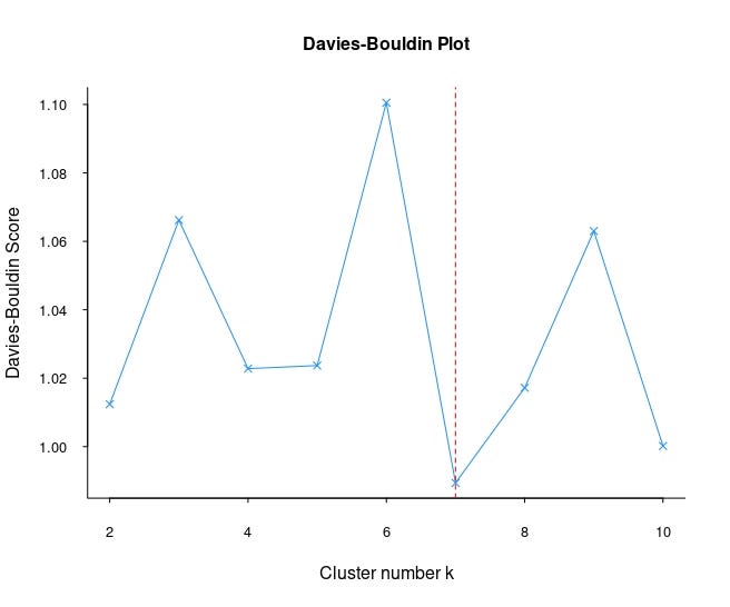
Unlike other methods, we see that Davies-Bouldin's suggestion for the number of clusters is 7. Although it gives different results in this data set, it can give more reliable results in other data sets. For this reason, it would be useful to include the Davies-Bouldin method in every clustering analysis.
Dunn Index
The Dunn index is a measure of the compactness and separability of the clusters in a clustering solution. It is calculated as the ratio of the minimum separation to the maximum diameter. [8]
The steps to perform Dunn Index are:
-
calculate minimum separation: the smallest distance between the observations from two different clusters.
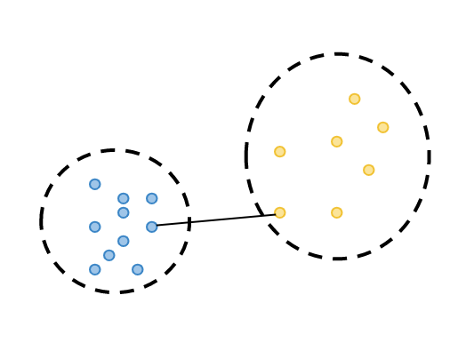
2. calculate maximum diameter: the maximum distance between the observations in the same cluster.
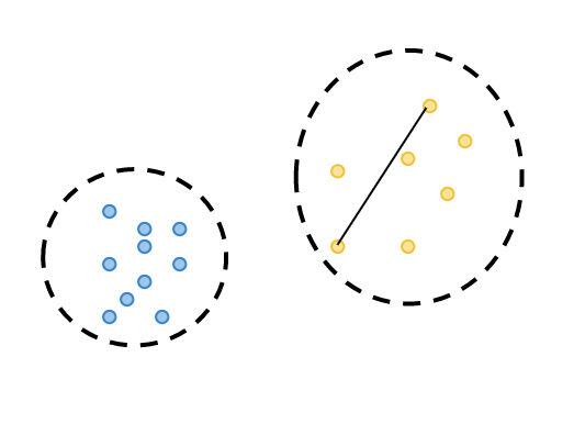
3. divide minimum separation by maximum diameter
The Dunn index ranges from 0 to infinity, with a higher value indicating a better clustering solution. A value of 1 indicates that the clusters are perfectly separated and perfectly compact, while a low value indicates that the clusters are either not separated or not compact.
Just like Calinski-Harabasz and Davies- Bouldin methods, there is no visualization function in R as for Dunn Index. For this reason, I will write a function that calculates and visualizes the Dunn Index values for the clusters 2 to 10 using the dunn function in the clValid package.
library(clValid)

fviz_dunn <- function(data) {
  k <- c(2:10)
  dunnin <- c()
  for (i in 2:10) {
    dunnin[i] <- dunn(distance = dist(data), clusters = kmeans(data, i)$cluster)
  }
  dunnin <- dunnin[2:10]
  plot(k, dunnin, xlab =  "Cluster number k",
       ylab = "Dunn Index",
       main = "Dunn Plot", cex.main=1,
       col = "dodgerblue1", cex = 0.9 ,
       lty=1 , type="o" , lwd=1, pch=4,
       bty = "l",
       las = 1, cex.axis = 0.8, tcl  = -0.2)
  abline(v=which(dunnin==max(dunnin)) + 1, lwd=1, col="red", lty="dashed")
}

fviz_dunn(df)
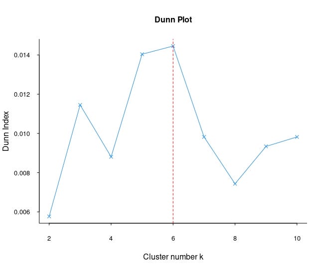
As the Davies-Bouldin methods, Dunn also suggested different cluster number. As I said before, each method may give different results for each data set. For this reason, it is useful to compare all methods in each clustering analysis.
Just like always:
"In case I don't see ya, good afternoon, good evening, and good night!"
References
[1] Steinley, D., & Brusco, M. J. (2011). Choosing the number of clusters in Κ-means clustering. Psychological methods, 16(3), 285.
[2] Halkidi, Maria, Yannis Batistakis, and Michalis Vazirgiannis. "On clustering validation techniques." Journal of intelligent information systems 17 (2001): 107–145.
[3] Rousseeuw, Peter J. Silhouettes: a graphical aid to the interpretation and validation of cluster analysis.Journal of computational and applied mathematics, 1987, 20: 53–65.
[4] Halkidi, M., Batistakis, Y., & Vazirgiannis, M. (2001). On clustering validation techniques. Journal of intelligent information systems, 17, 107–145.
[5] Tibshirani, R., Walther, G., & Hastie, T. (2001). Estimating the number of clusters in a data set via the gap statistic. Journal of the Royal Statistical Society: Series B (Statistical Methodology), 63(2), 411–423.
[6] Caliński, T., & Harabasz, J. (1974). A dendrite method for cluster analysis. Communications in Statistics-theory and Methods, 3(1), 1–27.
[7] Davies, D. L., & Bouldin, D. W. (1979). A cluster separation measure. IEEE transactions on pattern analysis and machine intelligence, (2), 224–227.
[8] Dunn, J. C. (1973). A fuzzy relative of the ISODATA process and its use in detecting compact well-separated clusters.