How to Interpret Linear Regression Output?
If you have a data set, you can easily build a multiple linear regression model with a little research on Google. But if you think it's all over with building a regression model, you're wrong.
In R, Python, and other programming languages, functions will output without any errors if you fill in their arguments and run them correctly. However, having an output never guarantees that it will be the correct output. For this reason, you should know how to interpret the outputs correctly, not only when building a regression model, but also in all analyzes you do. In this post of this series where I wrote about supervised learning, I wanted to touch on this issue. So, in this post I will try to explain how output of a multiple linear regression model should be interpreted.
It would not be wrong to say that the output of the regression model in R consists of four parts. These sections contain the model formula, descriptive statistics of residuals, information about coefficients, and information about the model. I will interpret each part in detail. But of course we need to build the model first. In this analysis, I will use Carseats dataset included in the ISLR package.
library(ISLR) # loading package for data set
df <- Carseats # assigning data set to an object

# building the model
model <- lm(Sales~Advertising+Price+Age+CompPrice+Income+Population,data=df)

# model output
print(model)
Call:
lm(formula = Sales ~ Advertising + Price + Age + CompPrice +
    Income + Population, data = df)

Residuals:
    Min      1Q  Median      3Q     Max
-4.9081 -1.3166 -0.1916  1.1511  4.6979

Coefficients:
              Estimate Std. Error t value Pr(>|t|)
(Intercept)  7.128e+00  9.795e-01   7.277 1.87e-12 ***
Advertising  1.309e-01  1.512e-02   8.654  < 2e-16 ***
Price       -9.253e-02  5.053e-03 -18.312  < 2e-16 ***
Age         -4.499e-02  6.009e-03  -7.487 4.68e-13 ***
CompPrice    9.385e-02  7.841e-03  11.969  < 2e-16 ***
Income       1.308e-02  3.471e-03   3.770 0.000189 ***
Population  -4.914e-05  6.844e-04  -0.072 0.942788
---
Signif. codes:  0 ‘***’ 0.001 ‘**’ 0.01 ‘*’ 0.05 ‘.’ 0.1 ‘ ’ 1

Residual standard error: 1.929 on 393 degrees of freedom
Multiple R-squared:  0.5403, Adjusted R-squared:  0.5333
F-statistic: 76.99 on 6 and 393 DF,  p-value: < 2.2e-16
At the top of the output, in the section titled Call, we see the formula we set up while building the model. Sales is our dependent variable. Advertising, Price, Age, Sales, and CompPice are independent variables.
At the bottom of the model output, it gives a statistical summary of the residuals that represent the differences between the model's predictions and the actual observations. Residuals show how well the model did not fit. Minimum, first quartile (1Q), median, third quartile (3Q), and maximum residual values are presented.
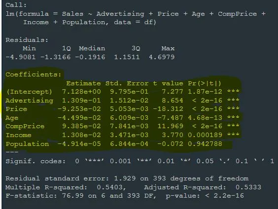
In the next part of the model output, we see the Coefficients. This section shows the coefficient estimates, standard errors, t-values, and p-values for each independent variable. Before explaining the each component of the Coefficients part, let me explain what they mean.

"Estimate" values of each variable represent the effect of that variable on the dependent variable.
"Std. Error" is a value that measures how accurate the estimation of each coefficient is. For the calculation, the variance of the error terms of the model and the covariance matrix of the coefficients are used. A higher standard error value indicates that the prediction is less accurate.
"t value" is a statistical value used to test whether a coefficient is nonzero. It is obtained by dividing the standard error of the estimate. A positive or negative t value indicates that the coefficient is nonzero. Large t values indicate that the coefficient is more reliable.
"p value" represents the probability that the coefficient is nonzero. p-value is obtained using a t-distribution table or statistical software for the given t-value and degrees of freedom. If the p-value is a small value (usually less than 0.05), it indicates that the coefficient is statistically significant and assumes nonzero. A large p value indicates that the coefficient is not statistically significant and we consider it close to zero.
Now, let me interpret each coefficient in detail:
Constant term Intercept represents the estimated initial value of the dependent variable when the influence of other independent variables is held constant. The estimate value here is 7.128e+00. This shows that the variable Sales is an estimated 7,128 units, holding the influence of other independent variables constant. Standard error, that is, the precision of the estimate, is 0.9795 units. t value (7.277) can be considered high and indicates that the coefficient is statistically significant. The p value (< 0.05) indicates that the coefficient is statistically significant.
Next coefficient is Advertising. The estimated value of this coefficient was calculated as 0.1309. For this reason, we can interpret that one unit increase in the Advertising variable causes an increase of 0.1309 units in the Sales variable when other variables are kept constant. The standard error is 0.01512 units. A high t value (8.654) and a low p value (< 2e-16) indicate that the Advertising coefficient is statistically significant and plays an important role in explaining the Sales variable.
Estimate value of our next variable, Price, was calculated as -0.09253. This indicates that a one-unit increase in the Price variable causes a -0.09253-unit decrease in the Sales variable, all other variables held constant. A high t value (-18.312) and a low p value (< 2e-16) again indicate that the Price coefficient is statistically significant and plays an important role in explaining the Sales variable.
When other variables are kept constant, it can be said that a one-unit increase in the Age variable causes a -0.04499-unit decrease in the Sales variable, since the Estimate value is -0.04499. Again, a high t value (-7.487) and a low p value (4.68e-13) indicates that the Age coefficient is statistically significant and plays an important role in explaining the Sales variable.
Since the next variables CompPrice and Income are statistically significant variables just like Advertising, Price, and Age, the interpretation of these variables will not differ from each other. For this reason, I think it makes sense to skip these variables and interprete Population variable.
The Estimate value of the Population variable is calculated as -0.00004914. Hence, when other variables are held constant, a one unit increase in the Population variable leads to a -0.00004914 unit decrease in the Sales variable. The low t value (-0.072) and high p value (0.942788) indicate that the coefficient of Population is not statistically significant. In this case, the Population variable does not play a significant role in explaining the Sales variable in a meaningful way.

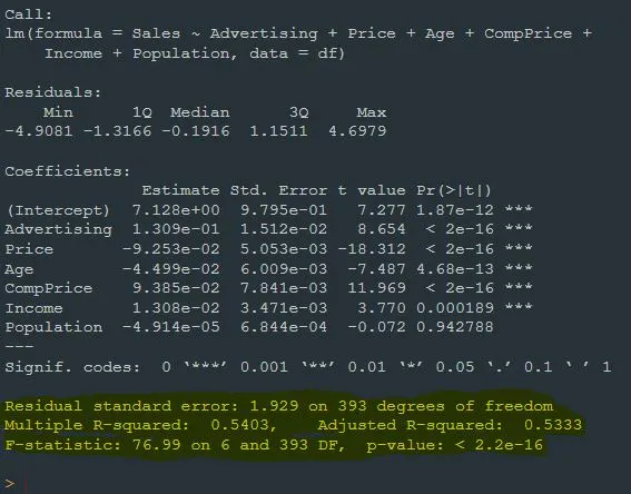
The next section in the regression model output is Residual standard error. This value measures how much the model's predictions diverges from the actual observations. A lower value means that the model fits the data better.Residual standard error here is 1.929.
Multiple R-squared represents the percentage of the variation of the dependent variable explained by the independent variables. It ranges between 0 and 1 and the closer it is to 1, the better the model explains the data. Here, the multiple R-square value is 0.5403. This indicates that the model explains 54.03% of the dependent variable. I will explain this in detail in the next post of this series.
Adjusted R-squared value is similar to the multiple R-square value, but is adjusted to take into account factors such as the number of independent variables and sample size. Adjusted R-square provides a fairer assessment, taking into account the complexity of the model. Here, the adjusted R-square value is 0.5333. Again, I will explain this in detail in the next post.
In the next section we see the F statistic value. The F statistic value mentioned here is actually a value obtained with the F test. The F test tests the validity of the model. Its hypotheses are as follows:
H₀: No linear relationship between dependent variables and independent variables
Hₐ: At least one independent variable affects the dependent variable.
Here, we see that the F statistic value obtained as a result of the F test is 76.99.
p value in the next section is entirely related to the F statistic. Based on the F statistic and the degrees of freedom determined by the estimated parameters and error terms of the model, the p value indicates whether the model is statistically significant. If the p value corresponding to the F statistic is less than the α significance level, Hₐ is rejected at the (1 — α)% confidence level, at least one coefficient is significant for the model. Therefore, the model is valid. We see that the model is also valid for this output.
Just like always:
"In case I don't see ya, good afternoon, good evening, and good night!"